Player Similarity Ratings

Intro

Every year at the NHL draft, hundreds of player comparisons are made between draftees and current NHL players. Beyond that, once players establish themselves as NHLers we still see comparisons being drawn between other players in the league. Traditionally, these comparables are made by people who watch both players play and see the similarities between their play styles and abilities.

Now as analytics have further seeped into the game and we have more stats for players than ever before, people have begun to create similarity scores that can describe how similar any two players are using their statistics. Here, I introduce my methodology for defining player similarity and explain other methodologies for defining player similarity.

There is a short summary of my methodology at the bottom alongside the applications and results for those not as interested in the technical aspects.

Past Research on Hockey Player Similarity

The majority of past work on player similarity uses some form of weighted euclidean distance between two players’ stat profiles.

The basis behind this is that if we think of players as existing in an n-dimensional space, where the number of dimensions is the number of stats we use to describe a player, we can then calculate what players are closest to each other in this space, and use that distance to decide which players are most similar through the euclidean distance formula.

The problem with simply taking the distance between players this way is that it treats every stat used as equally important in describing players. To break away from that limitation, people have imposed weights to each stat depending on how important they consider it, or if the stat is at a certain strength the weight is the proportion of time spent at that strength in the NHL. This is the approach taken by Emmanuel Perry and the Evolving Wild Twins.

Owen Kewell a member of the Queens Sports Analytics Organization employed a similar strategy to player similarity here. Where Owen’s methodology differs, is that he scaled all the statistics from 0-1 to avoid any issues that would arise from the varying magnitudes of the different stats; while Evolving Wild Twins used z-scores. Owen also weighted the previous three years of stats differently, but did not weight the individual stats by anything else; whereas Evolving Wild Twins weighed theirs by strength state, and Emmanuel Perry shows the use of weights but doesn’t specify how.

Lastly, Prashanth Iyer used nearly the exact same methodology as Owen Kewell in an article (paywalled) for The Athletic where he uses the components in Dawson Sprigings’ Goals Above Replacement model as dimensions but takes only the current year.

The last step in all of these scores is to find the farthest distance from an NHL player to the player you are trying to find and dividing each players distance by the max distance found then subtracting that value from one. Prashanth puts it nicely: “Thus, a player with 95 percent similarity would be 5 percent of the maximum possible distance away from the comparable player”.

My Approach

Like the approaches I’ve described above my methodology also uses euclidean distance and the same calculation at the end to determine a score; but, where my methodology differs is that I use the encoded values from an autoencoder (see below) as dimensions. This allows me to circumvent having to manually assign weights to each stat used in each players’ stat profiles or eliminate any stats I don’t think are “worthy” enough.

Autoencoders

Autoencoders are neural networks that take in data, pass it through a bottle neck, and then try to recreate the data that was originally passed as input.

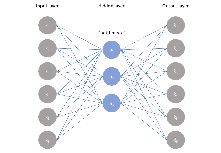
The idea is that I build a symmetrical neural network that tries to compress data, and then take the compressed data and turn it into its original representation.

I then train the autoencoder on data, and after that I can feed it new data and take the encoded values (values at the middle layer in the graph) and can use these new values to describe a player statistically.

Back to the Aproach

The autoencoder I used here takes all the freely available data for a player from evolving-hockey.com (meaning none of the RAPM or GAR numbers) then passes them to the bottle neck layer which is comprised of 4 nodes, and takes each nodes’ output and reconstructs the players stat profile from the four numbers attained in the middle layer. Because we take the values after they’ve been fully compressed inside the neural network, we call this the encoded values.

Since a player’s entire stat profile can be recreated from the encoded values, I calculate the euclidean distances from the encoded values instead of the original player stats. The idea is that the four numbers are able to describe a players entire stat profile, and the stats that are generally not that indicative of “uniqueness” have a smaller impact on the encoded values since the output nodes can estimate them easier without any priors; the same goes for stats that are highly correlated to one another.

I chose to use z-scores to standardize the data instead of scaling them 0-1 mainly out of personal preference.

Results

if for some reason a tableau dashboard doesn’t show up or it doesn’t fit on the screen you can go here to play around with the similarities

Click on any player listed on the list of players to see who they are most similar and least similar to. The slider on the top changes the number of players that appear in each graph taking the top x and bottom x players. The circles next to the player names also show how similar the player is to the selected player with the score corresponding to where the colour fits along the colour-bar at the top right.

The results show similarity scores for every centre in the 18-19 NHL season after training the autoencoder on centres from 14-15 to 17-18.

Autoencoders in Sports

Karun Singh has an amazing presentation on using autoencoders to find similar situations in a soccer game based on tracking data (here) and it is a big source of inspiration behind my approach to player similarity. In his research Karun uses an autoencoder to create 32 encoded values that represent a certain situation in a soccer match. He then uses the 32 values to find other situations that occurred which were very similar.

Applications

Aside from simple curiosity about who is similar to who, I can see two main applications for this from a management/analytics side.

1. Finding replacement player’s or trying to find a player that will fill a role in your team. For example, say player X is due to leave your team in free agency and while player X is not a superstar he serves a valuable purpose on your team and you want to find someone else who can work in that same role. The player similarity score would be very beneficial in creating shortlist of players that you could then get more information on before making a final decision as to who will replace player X.
2. Forecasting a player’s future. If you are able to find older players who were very similar to a player in their previous years you could use the similar players to project into the future. For example, player X and Player Y are both 20 and on your team but you can only pick one to keep on your team. You could find players who were very similar to X and Y when they were 20 and see how their careers panned out to help you make a decision. This is effectively the prospect cohort success model but applied to the NHL.

Future Directions

I intend this to be an example of how autoencoders can be used to describe how similar two players are to one another in a way that I think is better than how it has been done in the past. With that said there are two main things that I think should be included before anyone used the similarities for decision-making.

1. I only used 5 on 5 stats as inputs to the autoencoder, so while this does a good job at describing two players similarities at 5 on 5, it does not do a good job at the big picture analysis because two players that could be considered alike for their penalty killing abilities could be overlooked. Ultimately, the strength states you include in the model would be dependent on how you want to use the tool – because that is what analytics are, tools – if you want someone who is similar in all facets of the game I’d include stats at all strengths separated by strength, but if you just want someone who is similar in one aspect just include their stats at that strength (powerplay, even strength, penalty kill)
2. Explore how the results change when you have a different number of nodes in the middle layer that you use for encoded values. The higher the number of nodes you include in your middle layer the more information about players you’ll get, but as you add more nodes the value of each output may become more unequal and you won’t know how to weight them because this aspect of neural networks is a black box. Thus, you suffer a trade-off between a better description of a player for how much certainty you can have that the weights to each dimension should be equal

Summary

I built an autoencoder which uses every 5v5 stat available on evolving-hockey.com and calculated player similarity scores by taking the euclidean distance from the encoded stat profiles of each player and comparing each distance to the maximum distance found.