Clustering NHL Players by Usage

by: Nathan de Lara

Introduction

Burke’s Law is an autobiography by Brian Burke about his career in hockey and he describes a very interesting breakdown of how he wants to build his hockey teams. Burke places a player in each lineup spot that has the skills he wants each player to have.

I found this a very interesting and smart way to build a team, as it fits with how we think of players with having unique skillsets. If you want to play a certain way you need to build a team with players who have certain skillsets and can be used in the way you want to play them.

To explore this idea more, I set out to learn and classify players based on how they are used by their coaches. Through doing this I expect to learn more about player’s skills through the lens of their coaches and see how teams build their roster around where/how they want their players to be able to play.

I decided to cluster players based on usage stats and then evaluate those clusters to gain an understanding of basic categories into which players are placed. Each cluster should represent a unique way in which a player can be used by their team.

Methodology

I want to look at how players are used, not how things happen when they are used so I’m interested in their usage stats. Evolving Hockey’s public Zones table contain counts and other representations of where players started shifts by zone and their time on ice (there are other stats too but only these are relevant to measuring a player’s shifts starting conditions) . Their subscriber QoC and QoT tables contain the same above measures but for their average teammate and competition.

Variables

I pick the following variables:

• (QoC) TOI% : measures the proportion of ice time a player’s competition are given of their opposition’s total time at even strength
• (QoC) xGar Differential per 60 : the average xGar differential of a player’s competition
• (QoT) TOI % : measures the proportion of ice time a player’s on-ice teammates are given of their team’s total time at even strength
• (QoT) xGar Differential per 60 : the average xGar differential of a players on-ice teammates
• (Even Strength Zones) TOI%: the proportion of a team’s even strength ice team that a player gets
• (Even Strength Zones) OZS%: the percent of a player’s shifts that begin with them in the offensive zone
• (Even Strength Zones) DZS%: the percent of a player’s shifts that begin with them in the defensive zone
• (Even Strength Zones) NZS%: the percent of a player’s shifts that begin with them in the neutral zone
• (Power-play Zone) TOI%: the percent of how much time of a teams total power-play time is given to a player
• (Shorthanded Zone) TOI%: the percent of how much time of a teams total shorthanded penalty-kill time is given to a player

Given the stats we have, I want to learn how players are used by coaches. I chose stats that best represented what opportunities their coach gave them in the game. I excluded total time on ice and average time on ice stats because percentages encapsulate nearly the same significance and are more reflective of what I was looking for. I excluded percentage of on the fly shift starts in the interest of keeping dimensions low and it can be directly computed with DZS%, OZS%, and NZS%. I excluded the zone start stats for power-play and penalty-kill strengths because teams normally have squads that they send out regardless of zone so it would not give much information.

Dimension Reduction

Since I am looking to find groups within my data I used UMAP to project my data into two dimensions. When clustering data UMAP has shown to be a strong tool in reducing dimensions and into an embedding that can be more conducive to clustering as shown in their example of applying UMAP to the MNIST digit dataset in hopes of clustering with DBSCAN

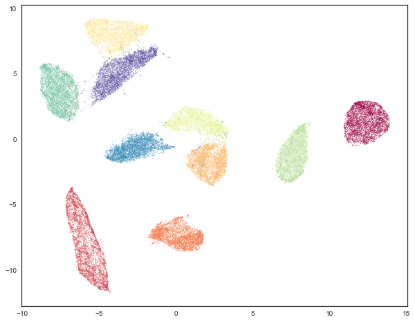
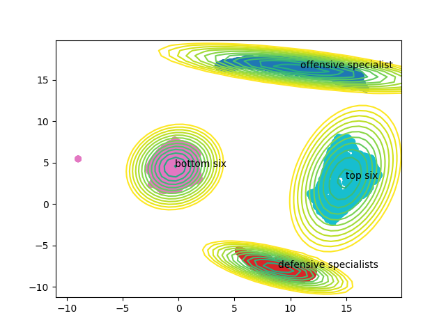
After applying UMAP to forward single season stats from the 08-09 to 21-22 season we find the embedding below:

Clustering

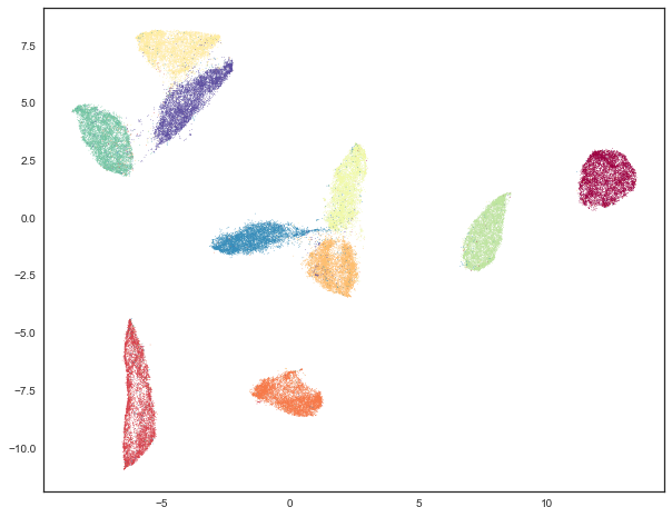
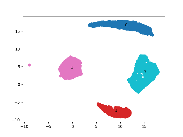
From the embedding we can see that there are four clear clusters that UMAP has sorted our players into. given the unique shapes in the embedding I chose to use Gaussian Mixture Modelling which aims to find multiple distributions within the data and returns a distribution to which each point belongs. Thee distributions are overlayed over the data on the table below

Cluster Analysis

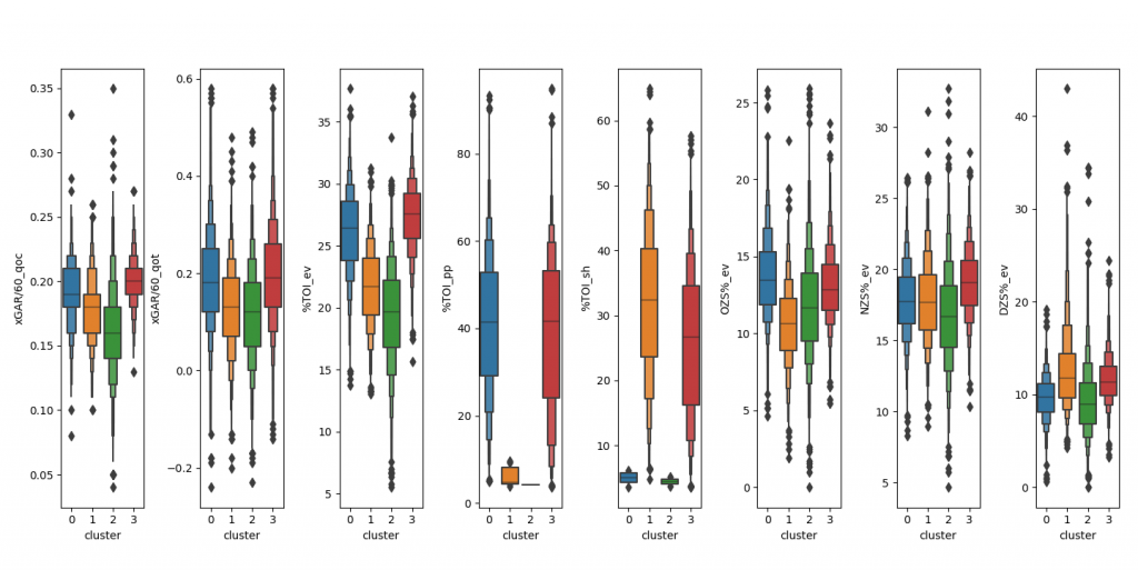
Graphing each clusters average in the original stats we see four clear statistical makeups

• Top Six: these players face good competition with good teammates and are deployed in all situations all over the ice
• Bottom Six: these players face below average competition with below average teammates and while getting used in all situations all over the ice they get used much less often than every other cluster. They are the jack of all trades, but seemingly master of none
• Defensive Specialists: These players face slightly below average competition with worse teammates than their opposition and get a lot of penalty-kill and defensive zone start opportunities
• Offensive Specialist: These players face above average competition with better teammates and have get a lot of power-play and offensive zone start opportunities

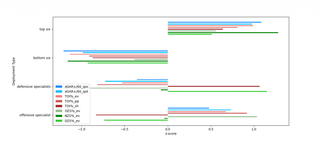
below is a chart showing how each clusters distribution compares to the other clusters in each stat

The labels also make sense within our 2d embedding of the players as offensive specialists and defensive specialists are opposite each other and so are top six and bottom six clusters. theres also offensive specialists closer to being top six players than others which corresponds with how we often do think of players as having a mixed toolset

Next, I wanted to look at how reliable these clusters are. If I say player X is used as an offensive specialist how likely am I to say that about him next year?

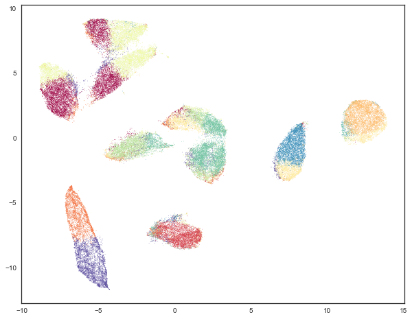
It turns our pretty likely, the plot below shows how players in clusters move between the clusters through different seasons. The size of the bars correspond to how many players fit that movement.

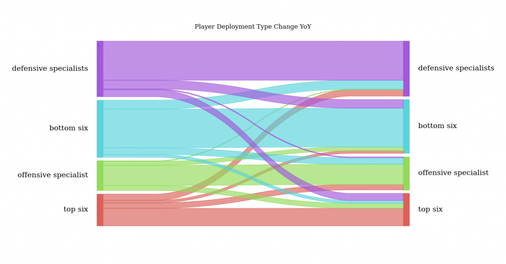
A defensive specialist is most likely to remain a defensive specialist but they can move to the bottom six or top six with seemingly equal likelihood (good defensively add some offensive skill and thats what you get) but rarely go to offensive specialist and this follows our understanding since it would be odd for a player to go from good defensively, bad offensively to bad defensively, good offensively (not to say it hasn’t happened though).

The movement for defensive specialists and offensive specialists is quite similar as if two sides of a coin which is a to be expected result.

For top six players when they do change deployment types, it is quite evenly spread out yet are slightly less likely to become a bottom six player than have an offensive/defensive specialist deployment.

Bottom Six player’s if they don’t remain in the same usage are likeliest to go to being a defensive specialist but rarely become someone who gets used like a top six player.

There appear to be many more defensive specialists than offensive specialists in the league so it seems that there are more players in the league who can penalty-kill and be reliable in the defensive zone compared to those who can play on the power-play and contribute in mainly offensive ways.